In real life situations, such as economics, biology, and many other fields, there are relationships among variables. This means that when an occurrence results or when a variable has the tendency to influence the other, the observations from the two variables are put together for analysis to establish the nature of relationships and the strength of the relationship. Thus, two-variable data demonstrates how results from a formula affect the overall output when any of the two input values changes.
Two-variable data is also called bivariate data in statistics- each value of one variable is coupled with a value of the other. Normally, it would be interesting to look into the possibility of a link between the two variables.
Rolling a Die and Throwing a Coin
We can draw a sample space for rolling a die and throwing a coin
| Coin/Die |
X1 = 1 |
X2 = 2 |
X3 = 3 |
X4 = 4 |
X5 = 5 |
X6 = 6 |
| Y1 = Head (H) |
P(H,1) |
P(H,2) |
P(H,3) |
P(H,4) |
P(H,5) |
P(H,6) |
| Y2 = Tails (T) |
P(T,1) |
P(T,2) |
P(T,3) |
P(T,4) |
P(T,5) |
P(T,6) |
Total Probability
There are 12 outcomes with equal probablity. X is the random variable of rolling a die. Y is the random variable of throwing a coin.
\( P(X_{i},Y_{j})= {1 \over 12}\)
Total Probability = \(\Sigma_{i=1}^{6}\Sigma_{j=1}^{2} P(X_{i},Y_{j}) = P(X_{1},Y_{1}) + P(X_{1},Y_{2})+.... + P(X_{6},Y_{1}) + P(X_{6},Y_{2})\) = 1
Expected Value
\(\mathbb{E}[XY] = \Sigma_{i=1}^{6}\Sigma_{j=1}^{2} X_{i}Y_{j}P(X_{i},Y_{j})\)
Since rolling a die and throwing a coin are both independent variables P(X_{i},Y_{j}) = P(X_{i})P(Y_{j})
\(\mathbb{E}[XY] = \Sigma_{i=1}^{6}\Sigma_{j=1}^{2} X_{i}Y_{j}P(X_{i})P(Y_{j})\)
Now you split the "i"s and the "j"s
\(\mathbb{E}[XY] = \Sigma_{i=1}^{6}X_{i}P(X_{i})\Sigma_{j=1}^{2} Y_{j}P(Y_{j})\)
You should be able to spot two expected values
\(\mathbb{E}[XY] = \mathbb{E}[X]\mathbb{E}[Y]\)
Rearranging this equation we can see that the Covariance is 0.
\(\mathbb{Cov}[X,Y] = \mathbb{E}[XY] - \mathbb{E}[X]\mathbb{E}[Y] = 0\)
This is a property of indepenence. We have shown that the covariance of two independent variables is 0.
Correlation
Variables that are strongly correlated imply that there is a relationship between them for example students who do well at Mathematics tend to do well at Physics.
Two variables can be either positively correlated, negatively correlated or no correlation.
The correlation coefficient r is used to determine the correction.
\(r = {\mathbb{Cov}[X,Y] \over \sqrt{\mathbb{Var}[X]}\sqrt{\mathbb{Var}[Y]}}\)
r is a value between -1 or 1. When r is positive, this implies positive correlation. When r is negative, the pair of data is negatively correlated.
If r is 0, then there is no correlation.
Positive correlation
For positive correlation most of the data is in the first or third quadrant. An example of positive correlation would be again Mathematics test result and Physics test. The centre of the 4 quadrants is \((\bar{x},\bar{y})\)
\[
\begin{array}{|c|c|c|}
\hline
\text{Quadrant} & x_{i}-\bar{x} & y_{i}-\bar{y} & [x_{i}-\bar{x}][y_{i}-\bar{y}] & \Sigma[x_{i}-\bar{x}][y_{i}-\bar{y}]\\
\hline
1 & \text{+ve} & \text{+ve} & \text{+ve} \\
\hline
2 & & & \\
\hline
3 & \text{+ve} & \text{+ve} & \text{+ve} \\
\hline
4 & & & \\
\hline
\end{array}
\]
\(\mathbb{Cov}[X,Y] = \Sigma [x_{i}-\bar{x}][y_{i}-\bar{y}] > 0 \)
The covariance is positive, hence the correlation coefficient is also positive.
Negative correlation
\[
\begin{array}{|c|c|c|}
\hline
\text{Quadrant} & x_{i}-\bar{x} & y_{i}-\bar{y} & [x_{i}-\bar{x}][y_{i}-\bar{y}] & \Sigma[x_{i}-\bar{x}][y_{i}-\bar{y}]\\
\hline
1 & & & & \\
\hline
2 & \text{-ve} & \text{-ve} & \text{-ve} & \text{-ve} \\
\hline
3 & & & \\
\hline
4 & \text{+ve} & \text{-ve} & \text{-ve} & \text{-ve} \\
\hline
\end{array}
\]
\(\mathbb{Cov}[X,Y] = \Sigma [x_{i}-\bar{x}][y_{i}-\bar{y}] < 0 \)
For the negative correlation, most of the data is in the second or fourth quadrant. An example of negative correlation could be hours playing video games and hours completing homework.
The covariance is negative, hence the correlation coefficient is also negative.
No correlation
For no correlation most of the data is evenly distribution in all four quadrants.
An example of correlation could possibly Maths test results and the time to complete a 5km race. There should be no relationship between the two variables.
\begin{array}{|c|c|c|}
\hline
\text{Quadrant} & x_{i}-\bar{x} & y_{i}-\bar{y} & [x_{i}-\bar{x}][y_{i}-\bar{y}] & \Sigma[x_{i}-\bar{x}][y_{i}-\bar{y}]\\
\hline
1 &\text{+ve} & \text{+ve} & \text{+ve} & \text{+ve} \\
\hline
2 & \text{-ve} & \text{-ve} & \text{-ve} & \text{-ve} \\
\hline
3 &\text{+ve} & \text{+ve} & \text{+ve} & \text{+ve} \\
\hline
4 & \text{+ve} & \text{-ve} & \text{-ve} & \text{-ve} \\
\hline
\end{array}
\(\mathbb{Cov}[X,Y] = \Sigma [x_{i}-\bar{x}][y_{i}-\bar{y}] = 0 \)
Since the points are evenly distributed in all quadrants the values in the last column will cancel itself out.
The covariance is 0, hence the correlation coefficient is also 0. Earlier we say that independent variables such as a die and a coin have no relationship, hence the covariance is 0.
Using vectors to show that |r|≤1
\( u = \begin{bmatrix} x_{1}-\bar{x} \cr x_{2}-\bar{x} \cr ... \cr x_{n}-\bar{x} \end{bmatrix} \)
\( v = \begin{bmatrix} y_{1}-\bar{y} \cr y_{2}-\bar{y} \cr ... \cr y_{n}-\bar{y} \end{bmatrix} \)
\( u.v = \begin{bmatrix} (x_{1}-\bar{x})(y_{1}-\bar{y} ) \cr (x_{2}-\bar{x})(y_{1}-\bar{y}) \cr ... \cr (x_{n}-\bar{x})(y_{n}-\bar{y}) \end{bmatrix} \)
vectors u, v and u- v form a triangle.
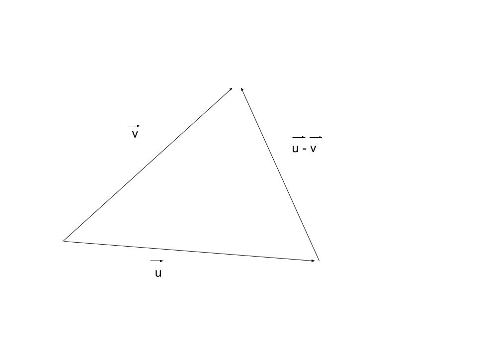
Using the cosine rule
\(|\vec{u}-\vec{v}|^2 = |\vec{u}|^2 + |\vec{v}|^2- |\vec{u}||\vec{v}|cos(\theta)\)
Recall from knowledge of vectors that \(|\vec{a}|^{2} = \vec{a}.\vec{a} \)
\((\vec{u}-\vec{v}).(\vec{u}-\vec{v}) = |\vec{u}|^2 + |\vec{v}|^2- |\vec{u}||\vec{v}|cos(\theta)\)
We can expand the dot product.
\(\vec{u}.\vec{u} -2\vec{u}.\vec{v}+\vec{v}.\vec{v} = |\vec{u}|^2 + |\vec{v}|^2- 2|\vec{u}||\vec{v}|cos(\theta)\)
Again using the property \(|\vec{a}|^{2} = \vec{a}.\vec{a} \)
\(|\vec{u}|^2 -2\vec{u}.\vec{v}+|\vec{v}|^2 = |\vec{u}|^2 + |\vec{v}|^2- 2|\vec{u}||\vec{v}|cos(\theta)\)
You can simplify the equation so that you end up with:
\({\vec{u}.\vec{v} \over |\vec{u}||\vec{v}|} = cos(\theta)\)
\(cos(\theta) \) is between -1 and 1, hence we have shown that:
\( -1 ≤{\vec{u}.\vec{v} \over |\vec{u}||\vec{v}|} ≤1\)
This is proof that the correction coefficient is between -1 and 1.
Two-Variable Data - Key takeaways
-
The covariance of independent variables = 0
-
Independent variables have a correlation = 0
-
a pair of data can have positive, negative or no correlation
-
Correlation coefficient r takes on values from -1 to 1.
